Setting up STATA database

• Obtain your file
• Ex: Open nlswork.dta. Give a command:

                    . use http://www.stata-press.com/data/r11/nlswork.dta

• Declare that data set is panel
• Indicate
• the name of the panel (idcode)
• the time variables (year)
• Both panel and time variables need to be numeric
• Then type:

                    . xtset idcode year

                    OR: Select Statistics -> Longitudinal/panel data -> Setup and Utilities -> Declare dataset to be panel data

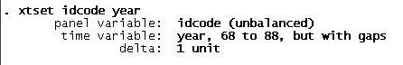
                    Output:

• "Unbalanced" idcode: gaps present among the id numbers
• "Year... but with gaps": no need to do anything
• Other considerations:
• Create a numeric code for any string panel variable (Ex: string date --> Stata date format
• Data should like this

          Panel ID     Time Variable     Var3     Var4     Var5...

               1                 1978                 ..           ..           ..   

               2                 1979

               3                 1980

               4                 1981

          (unique)        (Stata date)

          (numeric)       (numeric)

 Fixed Effects Regression

Entity Fixed Effects

Application:

• It helps to control for omitted variables that differ among panels, but are constant over time   

Example: Effect of 'experience' on 'earning'

• Here, earning (wage) obviously is influenced by factors other than experience (tenure), such as personality of the person, which can be assumed to stay constant over time
• With this assumption of fixed entity (other than 'experience') we can run a fixed effects regression with the following model: 

Then the model will be:

• ln(Wage) = intercept + b1*(TenureForEachPanel&Time) + b2*(UnobservedCharacteristicsForEachPanel) + ErrorForEachPanel&Time

• In STATA:
  

. xtreg ln_wage tenure, fe

• xtreg is used for panel data
• fe indicates other variables have fixed effect
• OR: select Statistics -> Longitudinal/panel data -> Linear models -> Linear regression (FE,RE,PA,BE)
  
• Output:
  
  

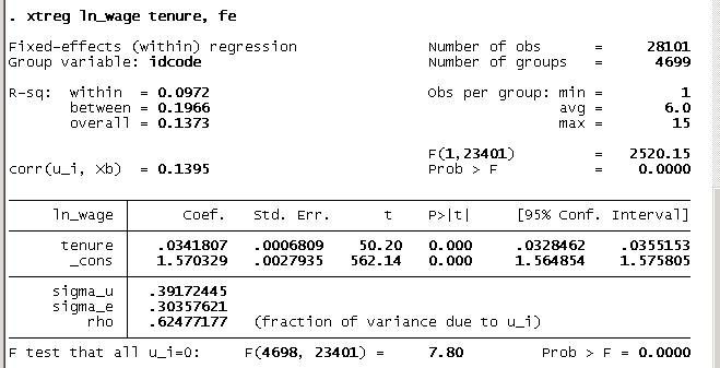
• The output shows you that it is a fixed-effects regression, with a group variable idcode.
• There is a total of 28,101 observations, and 4,699 groups (persons in this case)
• The observations per group, in this case year, ranges from 1 to 15. Plugging in the coefficients into the above model, we have:

• EstimatedLogWage = 1.57 + 0.034*(TenureForEachPanel&Time)

• This is equivalent to including n-1 dummy variables in the model, where n is the total number of panels in your data.

• Or, it may be more intuitive to exclude a constant and include n dummy variables.

• The dummy variables will absorb the panel variations that are consistent across time.

• In this data, it is not practical to create a dummy variable for each person, as there are close to 5000 people!

• But if you have a small number of panels, then you would have obtained the same coefficient by running a regular regression with dummy variables.

Time Fixed Effects

In this method, we assume that the unobserved effects vary across time rather than individuals (or persons - such as personality in previous example). Ex: national economy may impact everyone the same way but it varies across times (ex: in y1 it may be low and in y3 it may be higher). So to control for 'national economy' in a model, we can run time fixed effects regression model:

• Log(Wage) = (interceptForEachTime) + b1*(TenureForEachPanel&Time) + (ErrorForEachPanel&Time)

• So, the intercept includes the variation of time rather than panels. Estimation model will then be:

EstimatedLogWage = (TimeFixedEffects) + b1*(TenureForEachPanel&Time)

STATA Command:

. areg ln_wage tenure, absorb(year)

• areg is used to run fixed effect
• year is indicated as the variable to be absorbed
• OR Statistics -> Linear models and related -> Other -> Linear regression absorbing one cat. variable

STATA Output:

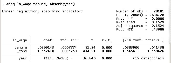
• By plugging in these coefficients, we have

EstimatedLogWage = 1.55 + 0.039TenureForEachPanel&Time

• As in the case of entity fixed effects, you can include t-1 dummy variables in the model, where t is the total number of years in the data.
• tabulate command with generate option creates a dummy variable for each year.
• Using asterisk (*) with yr, you can include yr1 through yr15.
• If you include a constant, then the constant takes the effect of the year that is ommitted.
• Here we purposefully exclude the constant.
• In the areg, the constant absorbed all the year's effects, whereas in the dummy version, you'll have an intercept for each year.

Dummy method (as opposed to areg)

. tabulate year, generate(yr)
. regress ln_wage tenure yr*, hascons

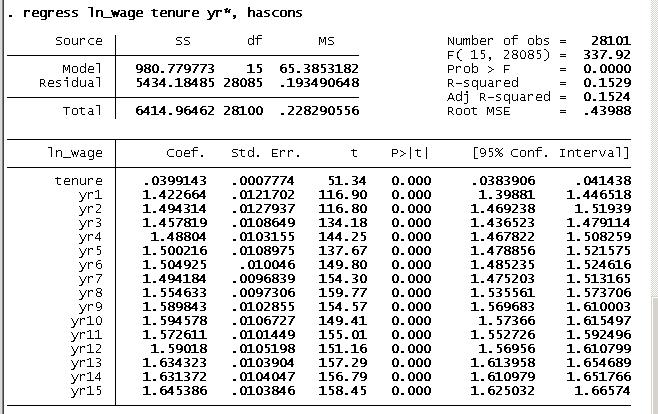
• Notice that the coefficient, standard error, and t-value of tenure are the same as in areg results.
• In time fixed effects model, we assumed that the slope for tenure is the same for all years but the intercept is different.

• If you think that there not only are effects that are different for each year, the effect of tenure would also be different for each year, you may run regressions for each year.

. sort year
. by year: regress ln_wage tenure

Random Effects Regression

Application:

• When some omitted variables may be constant over time but vary among panels, and others may be fixed among panels but vary over time

STATA

Stata's RE estimator is a weighted average of fixed and between effects models.

. xtreg ln_wage tenure, re

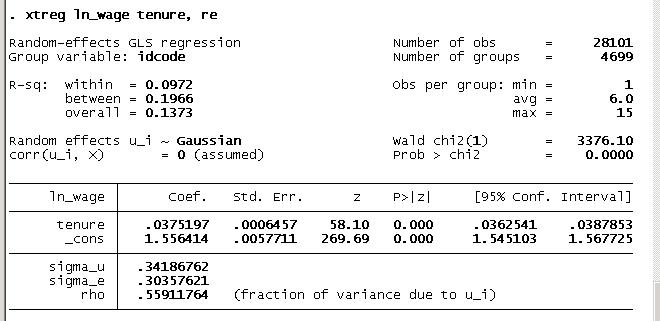
• Estimated regression outcome is:

• EstimatedLogWage = 1.55 + 0.0375TenureForEachPanel&Time

Choosing between Fixed-effect & Random-effect regressions

Perform Hausman test

• Save the coefficients from each of the models and use the stored results in the test

. xtreg ln_wage tenure, fe

. estimates store fixed

. xtreg ln_wage tenure, re

. estimates store random

. hausman fixed random

OR: Statistics -> Postestimation -> Tests -> Hausman specification test

• STATA Output: 

Between Effects Regression

Application

This model is similar to taking the mean of each variable in the model for each panel across time and running a regression on the collapsed data set of means

STATA

. xtreg ln_wage tenure, be

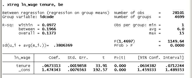
• In this data, some people's tenure information is missing
• In xt command, Stata will automatically exclude missing values from the computations.

Alternatively (more-work-version):

• Manually creating means with collapse, however, will not automatically exclude missing values.
• So we need to remove the cases with missing tenure before collapsing.

. drop if tenure == .
. sort idcode
. collapse (mean) meanLnWage=ln_wage meanTenure=tenure, by(idcode)
. regress meanLnWage meanTenure

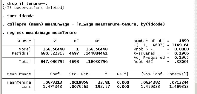
• The number of observations in the second regression matches the number of groups in xt regression.
• It created identical result as in the xt result above.

References

Contents adapted from: http://dss.wikidot.com/panel-data-analysis
- Stata Longitudinal/Panel-Data Reference Manual Release 11. Stata Press.
- Stock, James H. and Watson, Mark W. 2007. "Chapter 10 Regressino with Panel Data" in Introduction to Econometrics. Second Edition. Pearson Education, Inc.
- UCLA Academic Technology Services. Using xtreg. http://www.ats.ucla.edu/stat/stata/code/xt.htm ; retrieved August, 2010.
- UCLA Academic Technology Services. Stata FAQ: What is the relationship between xtreg-re, xtreg-fe, and xtreg-be? http://www.ats.ucla.edu/stat/stata/faq/revsfe.htm ; retrieved August, 2010.
03 Panel Data Analysis Methods